Plot genes with karyoploteR

How to visualise a set of genes accross the whole genome with karyoploteR

Dr. Cornelius Hennch, MD/PhD

Last updated on 20.05.2021 2 min read

How to visualize a set of genes across the genome

When analysing sequencing data, you might come across the situation in which you want to know the location of a set of genes across the whole genome. In this case, the karyoploteR package comes in handy. Here are three simple steps with which you can visualize a set of genes stored in a character vector.

1. Define the character vector with the genes of interest

# required packages
library(karyoploteR)

# genes you want to visualize
genes <- c('CD79A', 'CIITA', 'CSF2RB', 'DUSP2', 'HIST1H1E', 'IRF8', 'KLHL6', 'NFKB2', 'NFKBIE', 'NFKBIZ', 'PIM1', 'SOCS1', 'TNFAIP3', 'XBP1', 'IGLL5', 'NFATC2')

2. Get gene coordinates from Biomart

Choose the correct genome version, as coordinates can differ between the versions.

# 2. Biomart query (for hg19 = grch37) -----------------------------------------

ensembl <- biomaRt::useMart(biomart = "ENSEMBL_MART_ENSEMBL",
                            host = "grch37.ensembl.org",
                            path = "/biomart/martservice",
                            dataset = "hsapiens_gene_ensembl")

# get coordinates of the genes to visualize (corr_cn)
genes_coord <-
  biomaRt::getBM(attributes = c('chromosome_name', 'start_position',
                                'end_position', 'hgnc_symbol', "band"),
                 filters = 'hgnc_symbol',
                 values = genes,
                 mart = ensembl) 
  # constructs a GenomicRanges object from the bioMart query
genes_coord <- regioneR::toGRanges(genes_coord) 

# adds "chr" before chromosomes
seqlevelsStyle(genes_coord) <- "UCSC"

# check GRanges object
head(genes_coord)

# excludes duplicated CD79A entry
genes_coord <- genes_coord[-2]

## GRanges object with 6 ranges and 2 metadata columns:
##               seqnames            ranges strand | hgnc_symbol        band
##                  <Rle>         <IRanges>  <Rle> | <character> <character>
##   1              chr19 42381190-42385439      * |       CD79A       q13.2
##   2 HG1350_HG959_PATCH 42383025-42387277      * |       CD79A       q13.2
##   3              chr16 10971055-11026079      * |       CIITA      p13.13
##   4              chr22 37309670-37336491      * |      CSF2RB       q12.3
##   5               chr2 96808905-96811179      * |       DUSP2       q11.2
##   6               chr6 26156559-26157343      * |    HIST1H1E       p22.2
##   -------
##   seqinfo: 9 sequences from an unspecified genome; no seqlengths

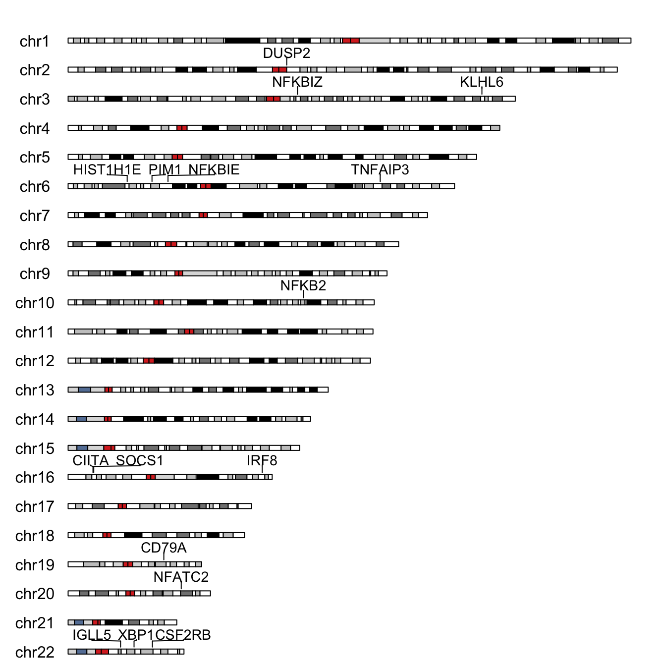
3. Plot with plotKaryotype + kpPlotMarkers

# just the chromosome ideograms
kp <- plotKaryotype(genome = "hg19", chromosomes =  "autosomal")

# add markers
kpPlotMarkers(kp, data = genes_coord,
              labels = genes_coord$hgnc_symbol,
              text.orientation = "horizontal",
              r1 = 0.5, cex = 0.9)

Just open and close the PDF device around the plot function calls in order to save it.

pdf("karyoplot.pdf")
kp <- plotKaryotype(genome = "hg19", chromosomes =  "autosomal")

kpPlotMarkers(kp, data = genes_coord,
              labels = genes_coord$hgnc_symbol,
              text.orientation = "horizontal",
              r1 = 0.5, cex = 0.9)
dev.off()

Voilà!

The whole documentation of the karyoploteR package can be found here.

Rmarkdown file with the whole source code can be found on Github.

R Visualisation